Spatial Rectification Algorithm

This chapter describes the algorithm used in the function rectify_dataset() of module xcube.core.resampling. The function geometrically transforms spatial data variables of a given dataset from an irregular source grid mapping into new data variables for a given regular target grid mapping and returns them as a new dataset.

Problem Description

The following figure shows a Sentinel-3 OLCI Level-1b scene in its original satellite perspective. In addition to the measured reflectances, the data product also provides the latitude and longitude for each pixel as two individual coordinate images. To the right, the absolute value of the gradient vectors of the latitude and longitude |(∇ lon)² + (∇ lat)²| are shown:

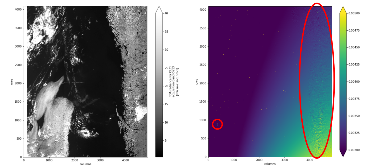
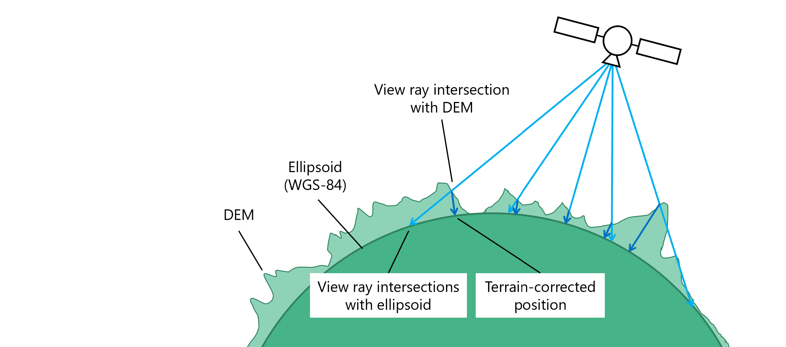
The given coordinates, latitude and longitude, are terrain corrected with respect to a digital elevation model (DEM) that approximates the Earth’s true fractal surface. Therefore, the gradient vectors are not monotonically varying over the scene, instead they represent the roughness of the DEM. Areas of high surface roughness are indicated by the red circles in the figure above. The figure below should explain the cause of the effect.

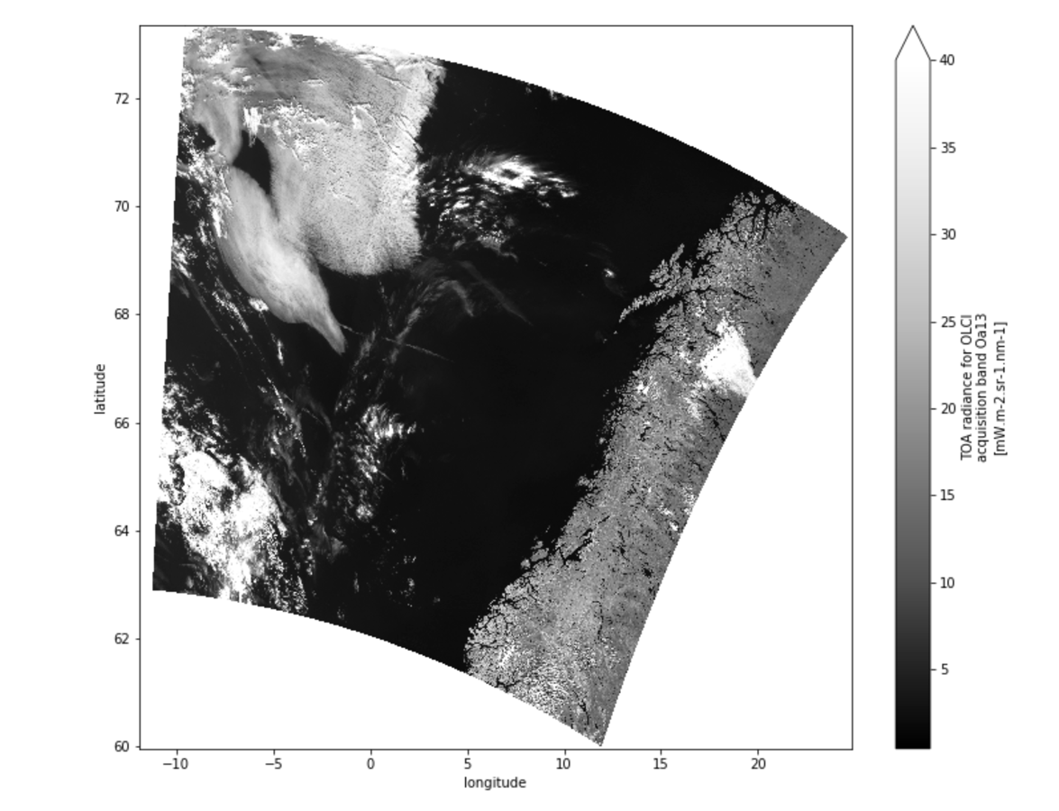
A rectification is the transformation of satellite imagery from its original viewing geometry into a target geometry that forms a regular grid in a defined coordinate reference system (CRS) with uniform spatial resolution for each pixel in each dimension. For the Sentinel-3 OLCI Level-1b scene above, the rectified measurement image for the geographic projection (CRS EPSG:4326) is shown here:

Algorithm Description

The input to the rectification algorithm is satellite imagery in satellite viewing perspective. In addition, two images – one for each spatial dimension – provide the terrain corrected spatial coordinates. Thus, for each source pixel we have a given spatial coordinate pair x,y, which is assumed to refer to a source image pixel’s center at i+½,j+½. The expected algorithm input is:

• N source measurement images;

• 2 source coordinate images (one for each spatial dimension) comprising terrain corrected coordinates x,y in units of the CRS for each pixel i,j;

The output produced by the algorithm is

• N target measurement images generated from source measurement images by projection.

• Target image geometry given as pixel size Δx=Δy and the coordinate offset of the upper left target image pixel x0,y0. Pixel size and offsets are given in units of the CRS.

• 2 target lookup images (one for each spatial dimension) comprising fractional source pixel coordinates i+½+u, j+½+v (explained below);

In the following, the CRS of the target and source is assumed to be the same. This is not a limitation, see remarks below.

While the gradient of the coordinate images, Δx and Δy per pixel, is generally not constant in the source image geometry, we demand that the target pixel size Δx = Δy = const for all pixels in the generated target images.

A fast and simple algorithm to perform the rectification is to visit each source pixel i,j, collect the spatial coordinates P = x,y, span two triangles between four adjacent coordinates, (P1, P2, P3) and (P2, P4, P3), and “paint” fractional source pixel coordinates into a new target lookup image. The lookup image can than be used to retrieve the pixel values from a source measurement image for a given pixel of the corresponding target measurement image, either by nearest neighbor lookup or by interpolation.

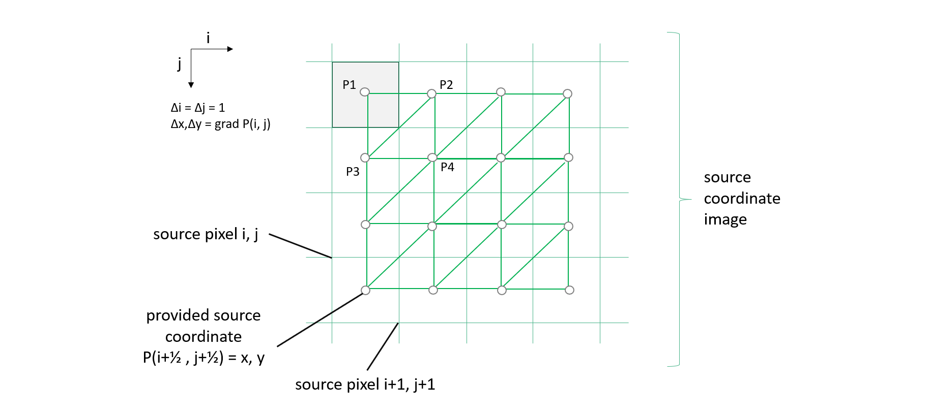
The true Earth surface is unknown in between any given coordinates points P(i+½, j+½) and its neighborhood, and there is no defined “best guess” for any point P(i+u, j+v) with 0 ≤ u ≤ 1 and 0 ≤ v ≤ 1. Hence, we use triangulation for its simplicity so that any in-between P is found by triangular interpolation.

From the coordinates (P1, P2, P3) of the first source triangle, the bounding box in pixel coordinates in the target image can be exactly determined, because the target grid is regular, P = x0 + i Δx, y0 - j Δy, for each target pixel i,j, target pixel size Δx,Δy, and x0,y0 being the coordinates of the upper left pixel at i=½, j=½. Given P and the plane given by (P1, P2, P3) the parameters u, v can be computed from triangular interpolation form P = P1 + u (P2 – P1) + v (P3 – P1). If 0 ≤ u ≤ 1, 0 ≤ u ≤ 1, u+v ≤ 1, then P is a point within the triangle.

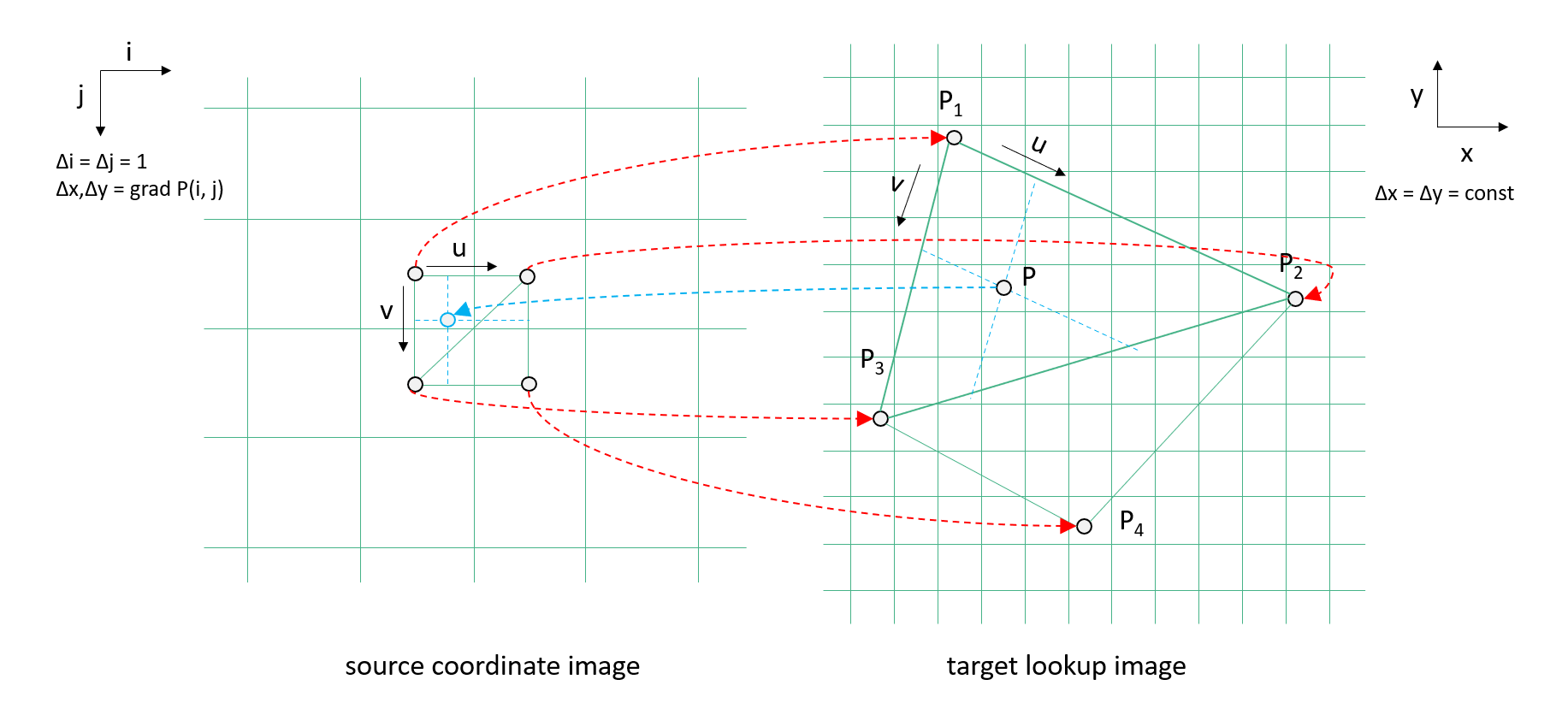
At the same time, u and v are the fractions of source pixel coordinate, i + ½ + u and j + ½ + v, which will be both stored in two target lookup images.

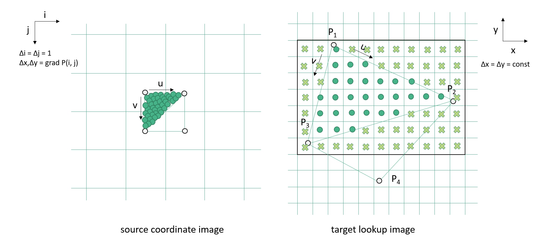
After all source pixels have been processed, the resulting target lookup images containing the fractional source pixel indexes, i + ½ + u and j + ½ + v, can be used to efficiently map a source measurement image V into the target measurement image. The pixel values of the source measurement image are given as V1 = V(i, j), V2 = V(i+1, j), V3 = V(i ,j+1), and V4 = V(i+1, j+1) here and are represented by different colour values, e.g., measurements such as radiances, reflectances, or higher level data variables:

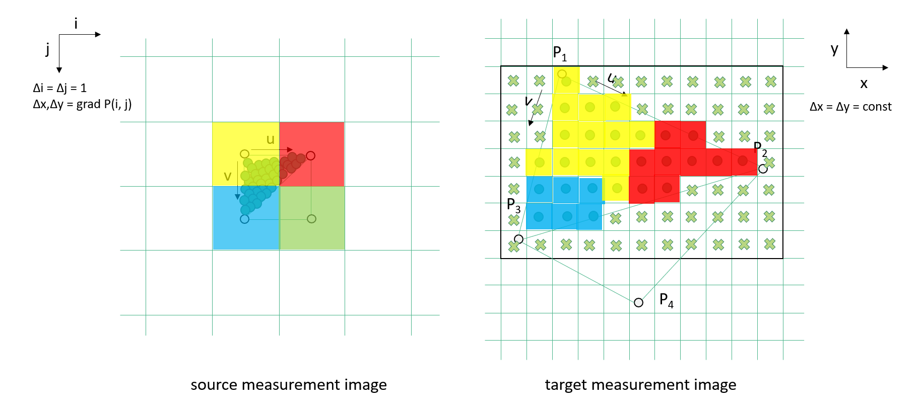
In the simplest case, as shown above, a nearest neighbor lookup is performed to determine the pixel value V for the target measurement image according to:

V = V2 if u > ½; V3 if v > ½; V1 else

The fractions u, v can also be used to perform the triangular interpolation between the three adjacent source measurements pixels. Note that the u, v were found from the three coordinate pairs that formed the original source triangle:

V = VA + u (V2 − V1) + v (V3 − V1)

Using bilinear interpolation between the four adjacent source measurements pixels also takes the fourth source coordinate P4 into account:

V = VA + v (VB − VA)

with

VA = V1 + u (V2 − V1)
VB = V3 + u (V4 − V3)

Remarks

(1) The target pixel size should be less or equal the source pixel size, so that triangle patches in the source refer to multiple pixels in the target image. However, if the target pixel size is distinctly smaller than the source pixel size, and the source has a low spatial resolution, results will be inaccurate, as curved source pixel boundaries need to be taken into account for many projections.

(2) If the target pixel size is greater than the source pixel size, target bounding boxes refer to single source pixels only. However, if the target pixel size is distinctly larger than the source pixel size, a prepended down-sampling or convolution of source images should be taken into account, e.g., using a Gaussian filter. Note, the algorithm can also be easily adapted to aggregate values of source pixels that refer to same target pixels.

(3) The algorithm description assumes that the source CRS and target CRS be the same. Different reference systems can be easily and efficiently supported by initially transforming each coordinate P(i, j) = (x, y) in the source coordinate images into the desired target CRS, i.e., P_new = transform_coord(P, CRS_S, CRS_T).

(4) If x, y are decimal longitude and latitude, and the north or south poles are in the scene, than the algorithm will fail. One can get around this problem by transforming source coordinates into a another suitable CRS first or by transforming longitude values x into complex numbers and optionally normalizing latitudes y to the same range from -1 to +1:

x’ = cos(x) + i sin(x)
y’ = 2y / π

(5) The algorithm can be rewritten to use bilinear surface patches comprising the adjacent four coordinates (P1, P2, P2, P4) instead of two triangles. The bilinear interpolation between the four coordinates is

PA = P2 + u (P2 − P1)
PB = P3 + u (P4 − P3)
P = PA + v (PB − PA)

Given that P is a known point on that surface the above can be rewritten as the two equations in u and v

0 = a + u b + v c + u v d
0 = e + u f + v g + u v h

with the solutions for u and v (from Wolfram|Alpha¹):

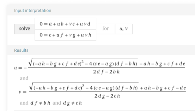
and with the differences

a = P1.x − P.x
b = P2.x − P1.x
c = P3.x − P1.x
d = P4.x − P3.x
e = P1.y − P.y
f = P2.y − P1.y
g = P3.y − P1.y
h = P4.y − P3.y

¹ Wolfram Alpha LLC, 2024. Wolfram|Alpha. https://www.wolframalpha.com/input?i2d=true&i=0+%3D+a+%2B+u++b+%2B+v++c+%2B+u++v++d%5C%2844%29+0+%3D+e+%2B+u++f+%2B+v++g+%2B+u++v++h+for+u%5C%2844%29+v (access April 8, 2024).